This post will be about Gaussian Processes and the design of a (afaik) new spatial kernel that was a pretty fun exercise. This exercise was motivated by a project I worked on the for Dutch Kadaster, so we’ll build the motivation for the new kernel through that application.
Gaussian Process Regression
Gaussian Process Regression (GPR) is lately turning up almost every commercial project I’m working on. I have a kind of love-hate relationship with them. Some things I like about Gaussian Processes:
- Considered a Machine Learning technique, which sells well. And selling projects is quite a big part of my work.
- Unlike Neural Networks, it yields very much interpretable results. I actually consider it not much more than a more flexible cousin of polynomial regression. I personally don’t like solving problems with black box Machine Learning techniques all that much, as they don’t give scratch my problem solving itch that much, and moreover require a lot of patience for training… (Not that I’m not blown away by recent OpenAI and Deepmind results though!). I wouldn’t even really call GPR Machine Learning if it didn’t sell so well.
Some things I don’t like about Gaussian Processes:
- Often doesn’t work so well in practise, often because challenges with length scales in multidimensional kernels and the tuning of such hyperparameters (coming up with way too long/short length scales)
- Bad computational complexity of $O(N^3)$ in the number of datapoints, but more fundamentally: GPR models spatial relationships in the covariance space, while I’m convinced that nature more naturally yields (sparse) relationships in precision space. The latter is more easy to work with computationally. I’m not very succesful of convincing other people of this view though. Work in progress…
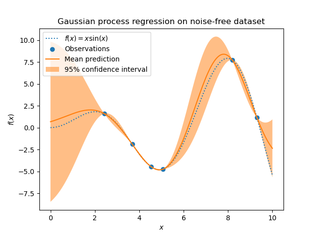
FYI: Google/ChatGPT is your friend to get acquainted with Gaussian Processes. I’ll not expand here and now on them… A first and very nice hit I encountered was this interactive application.
The Application: Kadastrale Kaart Next
‘Kadastrale Kaart Next’ (KKN) is a project of the Dutch Kadaster that also Sioux Mathware works on. The Dutch Kadaster governs the official maps and land administration of the Netherlands. With the KKN project, they want to make the current map more accurate, by refining the map through accurate land surveyor measurements. If the current map has $50.00$ meters between two points, but a land surveyor once measured $50.23 \pm 0.01$ m (currently hidden somewhere in a huge archive of millions of field sketches), then the two points are to be moved a bit, to exactly match that observation. But other observations need to be matched as well, so a whole neighborhood of points may move along as well. The mathematical theory of all this geodesy is called ‘adjustment theory’, and is described for example in the Dutch “Handleiding voor de Technische Werkzaamheden van het Kadaster” (HTW), of which an old 1938 version can be found here. The KKN project uses largely the 1996 update to that the HTW. This is a lot newer, but before the booming techniques like Gaussian Processes and/or HPC with sparse linear algebra. More details on the KKN project can be found in one of my few formal publications in the proceedings to a land surveyor conference.
Fundamental to (iterative) adjustment theory is statistics and Bayes’ rule (though the HTW probably doesn’t mention it as such). Adjusting the current map to a more accurate map when a new observation is added is nothing more than updating a prior to a posterior. Uncertainties in this theory are typically described with (multi-variate) Gaussian distributions, which are completely captured by the mean and the covariance matrix. One should expect this uncertainty to have correlations between neighboring points (two corners of a parcel), but not so much between points that lie very far away (like Eindhoven and Groningen). The covariance matrix will have some 2D spatial relationship to it, and maybe it already starts to feel a bit like Gaussian Processes (or Gaussian Fields if you like, as we’re working in 2D here)…
The Baarda-Alberda matrix and other sparse covariance matrix issues
To a large extent, following the Bayesian update rule, will yield a covariance matrix that has spatial features similar to Gaussian Process Kernel Matrices, but it will not be exactly the same due to the organic/historical/random nature of points and observations in the Netherlands. However, there were a few times in the project where we did see a need to create a custom (spatial) covariance matrix (using a kernel) from scratch.
The first application is the Baarda-Alberda matrix. To start the process of updating the current Kadastral map through Bayes’ rule, we need our starting point, the current Kadastral map, also to be described by a probability distribution. The current Kadastral map is the logical candidate for the mean, but what do we take for the covariance matrix? The HTW suggests the Baarda-Alberda matrix, which is uses a triangular kernel function:
\[\Sigma(x, x') = \max \left(0, \sigma^2 \left(1 - \frac{r}{r_{max}}\right)\right)\]with $r = |x - x’|$. It is “triangular” as the covariance dies off linearly with distance, until it reaches $r_{max}$, beyond which it is zero. This was deemed nice, as this yields covariance matrices that are somewhat sparse (depending on $r_{max}$ of course), unlike a squared exponential. The HTW does not use this terminology of a ‘kernel’ function and does not make any connection to the theory of Gaussian Processes (which was not so common in 1996). And that might be the reason that there is a problem with this kernel/matrix: It is generally not positive semi-definite (PSD) for points in a 2D plane (when using the radially symmetric Euclidean distance for $r = |x - x’|$)! And positive definiteness is very much needed for a matrix to function as a covariance matrix. How can we get any guarantees on this? (Btw, I’ll often omit the ‘semi’ from positive definite out of laziness.)
On the positive defiteness of kernels
The answer lies in Bochner’s theorem. I must say I haven’t (and won’t) plow through all the theory and mastered it. So I’ll present it the way I understand it roughly, and I am happy to be corrected by any readers. Matrices generated from kernel functions are positive definite if the function is ‘positive definite’. And a function is positive definite if and only if, its Fourier transform (FT) is a positive real function. If we then take the square root of that positive FT and transform back through the inverse Fourier transform, and combine that with how a product becomes a convolution under the Fourier transform, we can understand that we can have a proper kernel if it is the results of some self-convolution. Perhaps in (sloppy) equation notation easier to understand:
\[f(x) \succ 0 \Leftrightarrow F(\omega) > 0, \forall \omega \Leftrightarrow F(\omega) = G(\omega)G(\omega) \Leftrightarrow f(x) = g(x) * g(x)\](“Self-convolution” is probably the same as autocorrelation (at least for symmetric functions), but I think “self-convolution” is more self-explanatory.)
And now we can understand why the triangular kernel is positive definite in 1D. The triangular kernel can be obtained as the self-convolution of a rectangle/block function. In particular, the Fourier transform of a block function is a $\text{sinc}$: $\text{sinc}(\omega) = \frac{\sin(\omega)}{\omega}$, and that of a triangle function is $\text{sinc}(\omega)^2 = \frac{\sin(\omega)^2}{\omega^2}$. This latter is indeed positive for all $\omega$. Also the default kernel to Gaussian Processes checks out: The squared exponential yields a squared exponential through the Fourier transform and is positive. And the convolution of squared exponentials (or Gaussians) corresponds to the summing of Gaussian random variables. The sum of Gaussian random variables is Gaussian again: A squared exponential is the self-convolution of another squared exponential.
And now we’ll take a bit of a leap of faith (because I haven’t properly checked) and conject that Bochner’s theorem (which applies to 1D), can be made to work in 2D such that self-convolving a function in 2D will yield a positive definite 2D function. For squared exponentials, which are happily radially symmetric, things work out nicely too. But what about extending the triangular function? The block function is the indicator function on the 1D unit disk. If we consider the indicator function on the 2D unit disk and self-convolve that, we get a bit of a more complicated integral (= calculating the area of a lens = intersection of two circles). Still, this area is not too difficult to be solved analytically:
\[f(r) = \begin{cases} \arccos(r) - r\sqrt{1-r^2},& \text{if } r\leq 1\\ 0, & \text{otherwise} \end{cases}\]This function is known as the ‘circular’ model in the cov.spatial R package. The formula looks a bit different due to some scaling and some flexibility in formulating in terms of arccos or arcsin. However, there is also a critical mistake in the R package documentation: the square root inside the arcsin doesn’t belong.
Now what’s the use of writing these posts in Jupyter Notebooks if we’re not going to run any code and make and plots, amirite?
%matplotlib inline
import numpy as np
import matplotlib.pyplot as plt
def circular(r):
    if r > 1:
        return 0
    else:
        return np.arccos(r) - r*np.sqrt(1-r**2)

rs = np.linspace(0, 2, 101)
plt.figure()
circs = [circular(r) for r in rs]
plt.plot(rs, circs , label='Circular')
plt.plot(rs, circs[0]*np.maximum(0, 1 - rs), label='Triangle')
plt.xlabel('Radius')
plt.legend()
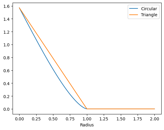
The circular model is going down quite linearly near the origin. However, it transitions a bit more smoothly to 0 around $r_{max} = 1$. This transition occurs curiously with a power of $p=1.5$, so not quite a quadratic transition. Also emperically we observed in the KKN project that this $p=1.5$ is crucial to PSD-ness.
And so this is the covariance matrix that we can start our KKN computations from. In practise, we also employ a method to make this kernel non-isotropic but dependent on a density estimate, as to get the maximum correlation length $r_{max}$ scaling with the inverse density (such that it becomes longer in rural areas and shorter in urban areas).
However, this kernel is not the new one I promised! To motivate that one, we move to the second (potential) application. Scalability of the iterative adjustment approach is a real challenge. The observations made by land surveyors create a huge graph of points where edges represent observations (like distance measurements between 2 points, or angles measured between three points). The sparsity pattern of this huge graph gets embedded into a huge matrix of (linearized) observations that are a precision-type matrix. When we invert that matrix, spatial correlation trends manifest that do not have a clear finite correlation length, but rather have some exponential decay with distance. (I might expand on the very interesting connection between (stochastic) partial differential equations and the Matern-class of GPR kernels in a later post).
This means, that our iterative procedure requires us to bring in more and more correlated points into the computations, which makes computation times explode. To keep the linear systems (core to any Bayesian statistics with MV Gaussian probabilities) small, we can truncate small correlation values to zero. However, truncation conflicts with that $p=1.5$-smooth transition to zero correlations that we encountered before. Truncating indeed generally breaks positive definiteness. One way to fix this is to project/scale the matrix back into the positive-definite cone. However, a particularly interesting idea that I found to this sparsity-enforcing strategy lies in a theorem I only recently learned about: The Schur product theorem. This states that the Hadamard (= element-wise) product of two positive definite matrices is also positive definite. (One of the simpler proof actually runs through statistics and uncorrelated random variables.) So rather than truncating values in a covariance matrix, we can get an alternative sparse approximation by multiplying with another covariance matrix (“the sparsifying matrix”) that has a finite correlation length, like ones created with the circular model shown previously. And now comes our “need” for a new kernel function: One would like “the sparsifying matrix” to be as close as possible to 1 for small distances, as to not modify the original matrix too much there. And one might find that the circular model, like the triangular function, decays too quickly at the origin (where it is non-smooth in fact), as it decays linearly.
Requirements for a new kernel
And so, after much ado, we get some requirements for a new kernel function:
- Positive definite (in 2D)
- Radial symmetry (in 2D)
- Finite support / correlation length
- Flat near the origin (= derivative of 0)
- Simple analytical formula
The kernel candidates we encountered till now score as follows:
| Kernel | Indicator on disk | Squared Exponential | Triangular | Circular |
|---|---|---|---|---|
| Positive definite (in 2D) | x | x | ||
| Radial symmetry (in 2D) | x | x | x | x |
| Finite support | x | x | x | |
| Flat near origin | x | x | ||
| Simple analytical formula | x | x | x | x |
So how can we achieve flatness near the origin? The reason that the circular model has a cusp at the origin can be understood the same way the triangular function has a cusp at the top. When we consider the triangular function as a self-convolution of a block function, it is the discontinuity of the block function that yields the cusp. If we self-convolve two triangular functions, we get a higher order B-spline ‘bump’ which is smoother allround, including at the top. So we’ll try and construct a new kernel by self-convolving - in 2D - a function with finite support that does not have a discontinuity at $r_{max}$ but goes to zero more smoothly.
Some first tries with numerical integration
Some first candidates for such a function were the triangular function itself, as well as the circular model obtained before. We will show, using numerical integration (scipy.integrate.dblquad) that we indeed get that flat top that we were looking for. First, we’ll show how numerical integration can indeed recover the circular model for our 2D self-convolution of the block function on a disk:
import scipy.integrate
def block(x, y):
    if x**2 + y**2 < 1:
        return 1
    else:
        return 0

ds = np.linspace(0, 3)
outs = np.zeros_like(ds)

for i, d in enumerate(ds):
    if d < 2:
        f = lambda x, y: block(x, y)*block(d - x, y)
        outs[i] = scipy.integrate.dblquad(f, -1, 1, -1, 1)[0] #x_low = d - 1 does not work?!

blocks = outs
Note that for a 2D convolution, we generally would have a double for-loop over a 2D integral. However, because of radial symmetry, we only need to sweep the distance between the two (shifted) copies of the input function, that then get multiplied and integrated. If we restrict the support of the candidate functions to be within $[-1, 1] \times [-1, 1]$ and ensure that they go to zero outside of their support, we can just integrate over that square. Also notice how the self-convolution of functions that go to zero at $r=1$ will go to zero only at center distance $d = 2$. But because I think it is nice to have a kernel that goes to zero at 1, you’ll see me rescale $d/2 \to r$ here and there…
plt.figure()
plt.plot(ds/2, blocks[0]/circular(0)*np.array([circular(d/2) for d in ds]), '-', label='analytical')
plt.plot(ds/2, blocks, '.', label='dblquad')
plt.legend()
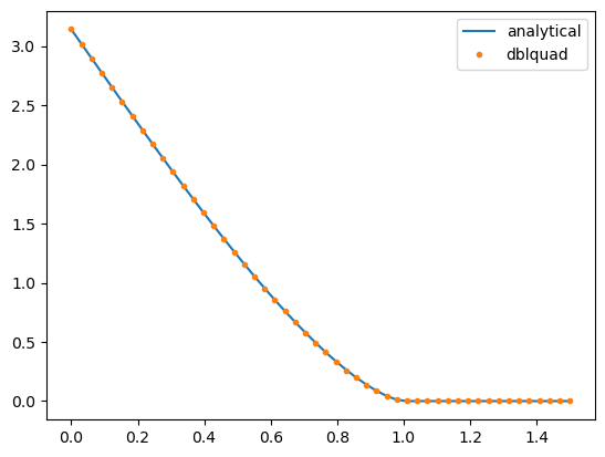
Scorcio! Let’s try with the triangular/conical and circular functions
# Triangular/conical
def cone(x, y):
    r = np.sqrt(x**2 + y**2)
    if r < 1:
        return 1 - r
    else:
        return 0

outs = np.zeros_like(ds)

for i, d in enumerate(ds):
    f = lambda x, y: cone(x, y)*cone(d - x, y)
    outs[i] = scipy.integrate.dblquad(f, -1, 1, -1, 1)[0]

cones = outs

# Circular
def circ(x, y):
    r = np.sqrt(x**2 + y**2)
    return circular(r)

outs = np.zeros_like(ds)

for i, d in enumerate(ds):
    f = lambda x, y: circ(x, y)*circ(d - x, y)
    outs[i] = scipy.integrate.dblquad(f, -1, 1, -1, 1)[0]

circs = outs
plt.figure()
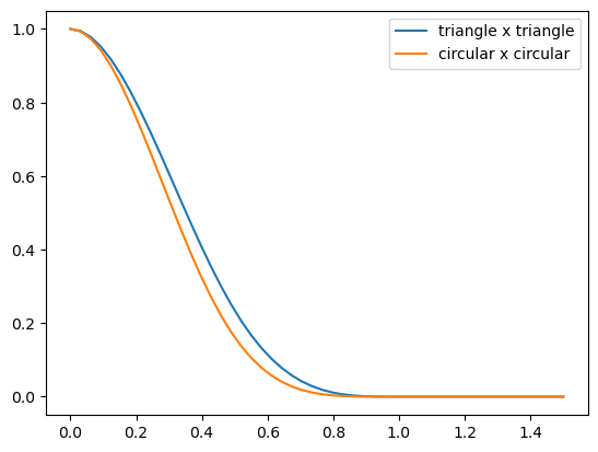
plt.plot(ds/2, cones/cones[0], label='triangle x triangle')
plt.plot(ds/2, circs/circs[0], label='circular x circular')
plt.legend()
plt.figure()
plt.plot(2-ds, blocks/blocks[0], label='block x block')
plt.plot(2-ds, cones/cones[0], label='triangle x triangle')
plt.loglog(2-ds, circs/circs[0], label='circular x circular')
plt.xlabel('1 - r')
plt.legend()
plt.grid()
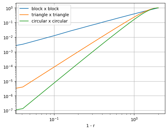
Hooray, we have managed to construct kernels with finite radius that are also smooth at the origin. We also see that smoothness at the top goes hand in hand with smoothness at the edge (which is not beneficial for sparsity). In fact, the smoothness at the edge has changed from $p=1.5$ for the block self-convolution to $p = 3.5$ and $p=4.5$ respectively for the triangular and circular self-convolutions.
Analytical integration attempts through SymPy
The big remaining question is, can either of these two kernels be respresented with a reasonably simple formula, like the circular function? We give it a go with SymPy (as we did in a preceeding post ). Again, we first check whether SymPy can recover the circular function, like we tested for SciPy.
import sympy as sp
x = sp.Symbol('x', real=True, positive=True)
y = sp.Symbol('y', real=True, positive=True)
d = sp.Symbol('d', real=True, positive=True)
r = sp.Symbol('r', real=True, positive=True)
out = sp.integrate(sp.integrate(1, (x, d/2, sp.sqrt(1 - y**2))), (y, 0, sp.sqrt(1 - (d/2)**2)))
2*out.subs(d/2, r)
$\displaystyle - r \sqrt{1 - r^{2}} + \operatorname{asin}{\left(\sqrt{1 - r^{2}} \right)}$
Unfortunately, SymPy does not recognize that $\arcsin(\sqrt{1-r^2}) = \arccos(r)$ for $r > 0$, but pretty… pretty good nonetheless! We took the integral over Carthesian coordinates, but did mind to put the info on where the function goes to zero explicitly in, through the integrand limits (rather than defining a conditional function like in the numerical approach). I also played around with taking these kinds of integrals in polar coordinates, but with no success.
Let’s see what happens when we put in the triangular function into this 2D integral:
out_y = sp.integrate((1 - sp.sqrt(x**2 + y**2))*(1 - sp.sqrt((d-x)**2 + y**2)), (x, d/2, sp.sqrt(1 - y**2)))
out = sp.integrate(out_y, (y, 0, sp.sqrt(1 - (d/2)**2)))

out.simplify()
$\displaystyle \int\limits_{0}^{\sqrt{1 - \frac{d^{2}}{4}}}\int\limits_{\frac{d}{2}}^{\sqrt{1 - y^{2}}} \left(\sqrt{x^{2} + y^{2}} - 1\right) \left(\sqrt{d^{2} - 2 d x + x^{2} + y^{2}} - 1\right)\, dx\, dy$
SymPy can’t seem to do anything nice with this. We did the 2D integral in two steps, not only for code readability, but also for to be able to inspect the intermediate result:
out_y.simplify()
$\displaystyle \int\limits_{\frac{d}{2}}^{\sqrt{1 - y^{2}}} \left(\sqrt{x^{2} + y^{2}} - 1\right) \left(\sqrt{d^{2} - 2 d x + x^{2} + y^{2}} - 1\right)\, dx$
Already this one did not manage to get anywhere. And not all that surprising, with these square roots in the integrand. In the polar coordinates I got it a bit further at some point, getting results in terms of the cryptic Meijer’s G-function that I would hardly call a simple analytical formula. I don’t even dare to try the circular function with that $\arccos$ in the integrand… So I was stuck for a few days, until it hit me that I’m free to choose my function however I like. And I like to make SymPy’s life easy (as long as I don’t introduce discontinuity). So what if we get rid of the square root?
Success!
If we take the function \(g(r) = \begin{cases} 1 - r^2 ,& \text{if } r\leq 1\\ 0, & \text{otherwise} \end{cases}\) and self-convolve that in 2D, we get the following function (up to some scaling and input and output side)
out_y = sp.integrate((1 - (x**2 + y**2))*(1 - ((d-x)**2 + y**2)), (x, d/2, sp.sqrt(1 - y**2)))
out_y.simplify()
$\displaystyle - \frac{d^{5}}{60} - \frac{d^{3} y^{2}}{3} + \frac{d^{3}}{3} + \frac{2 d^{2} y^{2} \sqrt{1 - y^{2}}}{3} - \frac{2 d^{2} \sqrt{1 - y^{2}}}{3} + \frac{8 y^{4} \sqrt{1 - y^{2}}}{15} - \frac{16 y^{2} \sqrt{1 - y^{2}}}{15} + \frac{8 \sqrt{1 - y^{2}}}{15}$
out = sp.integrate(out_y, (y, 0, sp.sqrt(1 - (d/2)**2)))
out.simplify().subs(d, 2*r).simplify()
$\displaystyle - \frac{2 r^{5} \sqrt{1 - r^{2}}}{9} + \frac{8 r^{3} \sqrt{1 - r^{2}}}{9} - r^{2} \operatorname{asin}{\left(\sqrt{1 - r^{2}} \right)} + \frac{r \sqrt{1 - r^{2}}}{6} + \frac{\operatorname{asin}{\left(\sqrt{1 - r^{2}} \right)}}{6}$
A final bit of simplification, we do manually, to obtain the relatively simple function:
sp.acos(r)*(sp.Rational(1, 6) - r**2) + sp.sqrt(1-r**2)*(r/6 + 8*r**3/9 - 2*r**5/9)
$\displaystyle \left(\frac{1}{6} - r^{2}\right) \operatorname{acos}{\left(r \right)} + \sqrt{1 - r^{2}} \left(- \frac{2 r^{5}}{9} + \frac{8 r^{3}}{9} + \frac{r}{6}\right)$
Which has quite similar ingredients to our previous ‘circular’ model, namely some $\arccos$ and some $\sqrt{1-r^2}$ stuff. Let’s take a look at how it looks:
def new_kernel(r):
    if r < 1:
        return np.arccos(r)*(1/6 - r**2) + np.sqrt(1-r**2)*(r/6 + 8/9*r**3 - 2/9*r**5)
    else:
        return 0
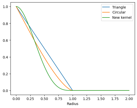
rs = np.linspace(0, 2, 1001)
plt.figure()
plt.plot(rs, np.maximum(0, 1 - rs), label='Triangle')
plt.plot(rs, [circular(r)/circular(0) for r in rs] , label='Circular')
plt.plot(rs, [new_kernel(r)/new_kernel(0) for r in rs] , label='New kernel')
plt.xlabel('Radius')
plt.legend()
rs = np.linspace(0, 1, 1001)
plt.figure()
plt.loglog(1-rs, [circular(r)/circular(0) for r in rs] , label='Circular')
plt.loglog(1-rs, [new_kernel(r)/new_kernel(0) for r in rs], label='New kernel')
plt.loglog(1-rs, (1-rs)**1.5, '--', label='$(1-r)^{1.5}$')
plt.loglog(1-rs, (1-rs)**3.5, '--', label='$(1-r)^{3.5}$')
plt.xlabel('1 - r')
plt.legend()
plt.grid()
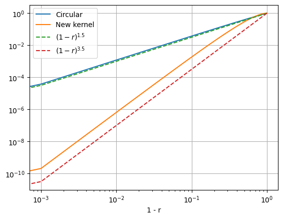
Eureka! Our new kernel checks all the boxes:
| Kernel | Indicator on disk | Squared Exponential | Triangular | Circular | Triangular x triangular | New kernel |
|---|---|---|---|---|---|---|
| Positive definite (in 2D) | x | x | x | x | ||
| Radial symmetry (in 2D) | x | x | x | x | x | x |
| Finite support | x | x | x | x | x | |
| Flat near origin | x | x | x | x | ||
| Simple analytical formula | x | x | x | x | x |
That’s all folks! Thanks for sticking around.
Acknowledgements
Shoutout to my colleagues Guus Bollen, Sven Hofmann and Juriaan Lucassen who collaborated with me on this stuff.
Related posts
Want to leave a comment?
Very interested in your comments but still figuring out the most suited approach to this. For now, feel free to send me an email.