Inequality constrained optimization

The topic of this blog post is close to my daily activities at Sioux Technologies. Over the past years, an optimization topic I have worked a lot on, is quadratic programming (QP), which has many control-related applications. A quadratic programming problem is an optimization problem with a quadratic cost function and linear inequality constraints (I have omitted equality constraints):

with $A$ a $C \times V$-sized matrix: $C$ constraints and $V$ variables, so $x$ lives in $\mathbb{R}^V$. In many applications, $H$ is a positive semi-definite matrix, such that the QP is a convex optimization problem.

Quadratic programs are, aside from linear programs, the simplest optimization problems with linear inequality constraints. A single linear inequality constraint $a_i x \leq b_i$ divides $\mathbb{R}^V$ into two half-spaces along a hyperplane, and eliminates half of $\mathbb{R}^V$ from being ‘feasible’. When dealing with a list of such constraints, we take the intersection of all those half spaces, such that the feasible set is also a convex set. In many application, we have with a feasible region which is compact (so it does not extend to infinity), and consequently is a polytope in $V$ dimensions.

%matplotlib inline

import numpy as np
import matplotlib.pyplot as plt

from matplotlib.patches import Circle, Wedge, Polygon
from matplotlib.collections import PatchCollection

def HalfPlane(a, b):
    a = np.array(a)
    
    # Ax <= b (fill the forbidden area)
    assert len(a) == 2
    
    if a[0] == 0:
        pl = np.array([-1000, b/a[1]])
        pr = np.array([1000, b/a[1]])
    elif a[1] == 0:
        pl = np.array([b/a[0], -1000])
        pr = np.array([b/a[0], 1000])
    else:
        p0 = np.array([b/a[0], 0])
        p1 = np.array([0, b/a[1]])

        pl = p0 - 1000*(p1 - p0)
        pr = p0 + 1000*(p1 - p0)
    
    pl2 = pl + 1000*a
    pr2 = pr + 1000*a
    
    points = np.array([pl, pr, pr2, pl2])
    return Polygon(points, True)

A = np.array([[1, 0], [-1, 0], [1, 1], [-1, -1]])
b = np.array([1, 1, 2, 2])

fig, ax = plt.subplots(figsize=(6, 6))

patches = []
for i in range(A.shape[0]):
    patches.append(HalfPlane(A[i, :], b[i]))

p = PatchCollection(patches, alpha=0.4, edgecolor='b', linewidth=3)
ax.add_collection(p)

plt.xlim(-4, 4)
plt.ylim(-4, 4)
ax.set_aspect('equal')

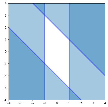
The above figure illustrates a set of 4 linear inequality constraints in a 2D space. Each individual linear inequality constraint eliminates a half-space (blue). The white rhombus at the center are all the points satisfying all constraints. The linear inequality constraints have defined a polytope (which in 2D is a polygon).

Quadratic programming methods

The classic book ‘Numerical Optimization’ by Nocedal and Wright has an excellent introduction to constrained optimization in chapters 12 - 16. In particular chapter 16 on quadratic programming has been of a lot of use to me in the past years. Two big schools of methods are outlined there: active set methods and interior point methods.

• Active set methods find their way to the optimal solution of the optimization problem along the edge of the feasible region/polytope. For every constraint, they keep track of a binary variable, whether that constraint is active ($a_ix = b$) or not ($a_ix < b$). In a basic active set method, at each iteration, either one constraint is added to the active set, or removed from the active set.
• Interior point methods find their way through the center of the feasible set. Constraints are never truly activated. The linear (in)dependency matter, is mostly of concern when using active set methods.

Linearly dependent constraints

In a lot of constrained optimization theory, such as in the book of Nocedal and Wright, the Linear Independency Constraint Qualificiation (LICQ) assumption is made, which simplifies both theory and algorithms/software. On page 320 of Nocedal and Wright, Definition 12.4 states:

Given the point $x$ and the active set $A(x)$ defined in Definition 12.1, we say that the linear independence constraint qualification (LICQ) holds if the set of active constraint gradients ${∇c_i(x),i∈A(x)}$ is linearly independent.

The Nocedal theory applies to nonlinear constraints. For linear inquality constraints, these constraint gradients $\nabla c_i(x)$ are just the vectors $a_i$. Note that the LICQ concept is something that applies to a point $x$ and not to - for example - the entire set of linear inequality constraints.

The importance of these conditions are evident when considering active set methods. When an active set method encounters a point at which the LICQ condition does not hold, there is a risk of it not converging properly, and that is rather starts cycling. Care must be taken!

Cycling, degeneracy, ties are all keywords related to LICQ conditions not holding. Other terminology that I have come across is linearly (in)dependency of constraints. And my experience is also that this latter terminology can lead to a lot of confusion. Linear dependency of constraints is different from linear dependency of vectors or rows/colums of constraint matrix $A$. The simplest possible example to explain this is a very common one: symmetric lower and upper bounds on a 1D constrained optimization problem: $-1 \leq x \leq 1$

In standard $Ax \leq b$ form, this is equivalent to \(A = \begin{bmatrix} 1 \\ -1\end{bmatrix}, \qquad b = \begin{bmatrix} 1 \\ 1 \end{bmatrix}\)

Matrix $A$ above is not of full rank, and the rows are linearly dependent. However, these constraints do not pose any LICQ difficulties, because the two constraints can never be activated at the same time as one would have $1 = x = -1$!

If the above are not ‘linearly dependent constraints’, then what are? We better move up 1 dimension to 2D. Below is an example.

A = np.array([[1, 0], [-1, 0], [1, 1], [-1, -1], [2, 1]])
b = np.array([1, 1, 2, 2, 3])

fig, ax = plt.subplots(figsize=(6, 6))

patches = []
for i in range(A.shape[0]):
    patches.append(HalfPlane(A[i, :], b[i]))

p = PatchCollection(patches, alpha=0.4, edgecolor='b', linewidth=3)
ax.add_collection(p)

plt.xlim(-4, 4)
plt.ylim(-4, 4)
ax.set_aspect('equal')

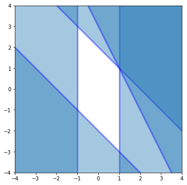
In the above figure, point $(1, 1)$ is a point at which the LICQ condition does not hold. At that point, 3 out of the 5 inequality constraints are active (the inequality $\leq$ is in fact an equality $=$):

In this case, the matrix $A_{act}$ is again not of full row-rank, and in this case this is problematic.

A more geometric interpretation of degeneracy is 3 lines in 2D intersecting at a single point. This can be generalized to $n$ hyperplanes in $n-1$D intersecting at a single point, or even to $n$ hyperplanes in $m$ dimensions intersecting with a dimensionality of $n - m - 1$ or higher (where a point is a non-empty 0D set).

One might argue that linear dependency is perhaps a trivial matter in 2D, as in general (and also in the example) some of the problematic constraints will be redundant: The feasible set would not change (/grow) if we omit the right constraint. (Redundant constraints is a topic on the backlog for future blog posts.) If one removes all redundant constraints in 2D no linear dependency issues will remain. This is not true in 3D or higher, as the following example illustrates.

Both the octahedron and icosahedron are polytopes in 3D with vertices at which >3 (hyper)planes intersect. At each of the vertices, the LICQ condition does not hold.

Whereas the LICQ condition holds for a point, in common terminology, what we mean when we say that a feasible set $Ax \leq b$ is linearly dependent is that there is a point in the feasible set at which the LICQ condition is not satisfied.

Prevalence of linearly dependent constraints

The above exposition shows that linear dependency of constraints is a matter involving both $A$ and $b$. For random constraints (or for example, fixing $A$ and choosing random $b$), the probability of having linear dependency problems is 0. So, one might think this is rare in practise and that the LICQ assumption is reasonable. The central point of this blog post is that I have encountered such linearly dependent constraints multiple times in practise. They are not that rare at all. This causes simple implementations of active set methods headaches. For example, they get stuck in infinite loops of activating and deactivating constraints at the problematic vertices and never converge to the true optimum.

Example

One particularly simple occurrence of linearly dependent constraints appears in setpoint/trajectories calculations of mechatronic systems. Setpoints are parametrised by polynomial or piecewise polynomial functions of time, and the dynamic limitations of the hardware are imposed as range constraints, velocity constraints, acceleration constraints and sometimes even higher orders.
Setpoint trajectories may be parametrized for example as 3rd degree polynomials like

The variables of the optimization problem would be the parameters $p_i$, so we’d have a 4D optimization space.

A range-constraint would be

A velocity constraint would be

Note that the $\forall$-part makes this a non-standard type of constraint. It is not simply of the form $g(p) \leq 0$ for some explicit function $g$. It is a non-linear constraint, but definitely not a simple one. Also this might be a topic for another blog post.
A common approach to deal with this tricky $\forall$ in practise, is to not require the constraint at all values $t \in [t_0, t_f]$, but only at a finite number of samples (often chosen uniformly spaced) $t_j$ with $j = 1..N$. With $N$ samples, we now get $N$ two-sided range constraints:

This can be rewritten into a matrix format using a Vandermonde-matrix

By sampling, we have replaced a complex non-linear constraint with $2N$ linear inequality constraints. A higher $N$ will take more computational effort, but will allow less constraint violation in between the sample points. For the remainder of the section, lets assume 10 sample points for a cubic polynomial trajectory. Note that the same approach can be taken for velocity and higher order constraints.

It is quite easy to show that these constraints suffer from linear dependency in some points of the feasible set. One particularly nasty point is the point

This trajectory is in the feasible set, and the range constraint is active at each of the $N=10$ sample points. 10 active constraints in a 4D space is definitely a matter of LICQ violation.
In combination with velocity and higher order constraints, other problematic points might exist as well, and one could do a brute force search for them by checking the ranks of a combinatorial number of submatrices. Again, perhaps a topic for a future post… In any case, the main point of this section is that it is quite easy to find real world applications with constraints that have LICQ violating points. Moreover, the LICQ violation point above, is not an exotic / funky looking setpoint profile at all. It is quite reasonable to be a solution or an intermediate iterate for some real world QP.

Handling linearly dependent constraints

Active set methods

So, what do Nocedal and Wright think of all of this?

• Chapter 13 on linear programming with the simplex method has a section titled ‘Degenerate steps and cycling’, which is exactly about the linear dependency issues we are dealing with. If no care is taken, active set methods can reach a linear dependent point and start cycling. The book states

  Cycling was once thought to be a rare phenomenon, but in recent times it has been observed frequently in the large linear programs that arise as relaxations of integer programming problems.

  This is not what we illustrated moments ago: Even small and quite common problems can face degeneracy. The section presents two mitigation strategies: a perturbation strategy and a lexicographic strategy.

• Chapter 16 on quadratic programming, in the section on active set methods, refers with respect to degeneracy and cycling to chapter 13, and even states

  Most QP implementations simply ignore the possibility of cycling.

  Again, this blog post tries to advocate this is a poor decision.

The perturbation strategy perturbs the vector $b$ by a small amount in every entry as to break the linear dependency. Nocedal and Wright argue that the perturbations are applied consistently throughout iterations, then this resolves all problems. The only challenge is to choose the perturbation amount large enough that numerical linear dependency is resolved, but small enough that the original problem is not perturbed too much. The lexicographic approach eliminates the choice of a perturbation size by assuming infinitesimal perturbation and doing proper bookkeeping.

Intermezzo: Sage for visualizing linear inequality constraints

Polytope representations

The previous section makes a nice bridge to a visualization tool for constraints in 3D, namely using the Sage Mathemathical software and in particular the Polyhedron functionality.
In 2D constraint visualization is quite easy, as we illustrated above. Drawing entire hyperplanes in 3D makes for a poor visualization with a lot of clutter. Linear inequality constraints define polytopes (= polyhedra in 3D) so ideally we would just visualize the vertices, edges and faces of that. However, I have not stumbled across a lot of tools to convert linear inequalities into vertices, edges and faces. It is not trivial, as it is not obvious from a list of inequality constraints which ones will intersect at a point which is feasible (though on the boundary) and which ones intersect outside of the feasible region. By the way, the other way around is much easier (for every face, define the appropriate linear inequality constraint).
The only tool I have stumbled upon that does this conversion (and visualization) is Sage. Before the discovery of that, I tried some voxel and levelset type of visualizations, but none of them show the boundary of the feasible set in a very crisp manner.

Before illustrating what Sage can do, one more remark about polytope representations. In general dimensions, two different ways of representing are

1. linear inequalities, or
2. extreme points which a compact polytope has a finite number of.

A convex set can be built up as all possible convex combinations of the extreme points. In 3D the vertices are the extreme points. Extreme points alone do not yet give the edges of the polyhedron which contribute to a nice visualization too though. I have not yet looked into the literature on whether there are any nice methods for conversion between linear inequalities and extreme points (and back) beyond brute force stuff of combinatorial complexity.

Sage code

To start off, I’m not an experienced Sage user, and what I managed to do below was a matter of copy-paste programming. First off, Windows is not supported by Sage, so I had to resort to an Ubuntu VM. From there, Sage can be imported as a Python package (after installing, for example from conda-forge), but the graphics rendering does not work out of the box in a Jupyter notebook. The quickest solution was to write the graphics to file and render the file with IPython.display.Image. Alternatively, one can play around with Sage in the browser using the Sage Cell Server and it seems that it can even be used with Jupyter Notebooks with a Sage kernel i.s.o. the Python kernel I’m using.

The core functionality of Sage I’m now interested in, is the Polyhedron class, which allows definition of a polyhedron in terms of linear inequalities (through the ieqs keyword argument). The documentation specifies that ieqs needs to receive a list of lists in [b, A] format to represent inequalities \(Ax + b \geq 0\)

import sage.all
from sage.geometry.polyhedron.constructor import Polyhedron

from IPython.display import Image

s = np.sqrt(2)/2

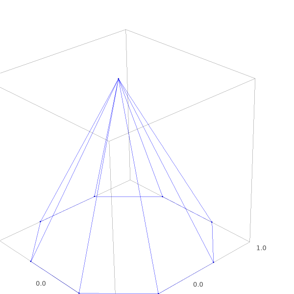
The polyhedron we create is an 8-sided pyramid. The top of the pyramid is a degenerate point. A point in 3D is uniquely defined by 3 intersecting planes. The pyramid top has 8 intersecting planes. One can imagine an active set ending up at this point, will have a hard time choosing the right direction to continue the search in. For a 100-sided pyramid, the challenge is even greater.

p = Polyhedron(ieqs=[[0,0,0,1], #Ground plane
                    [1, -1, 0, -1], #1st side
                    [1, 1, 0, -1],
                    [1, 0, -1, -1],
                    [1, 0, 1, -1],
                    [1, -s, s, -1],
                    [1, s, s, -1],
                    [1, s, -s, -1],
                    [1, -s, -s, -1]]) #8th side

g = p.plot(fill=False)
g.save('tmp.png', zoom=1.5, figsize=[6, 6])
Image(filename='tmp.png')

As the above code and figure show: we construct a polyhedron from inequality constraints, but Sage does render vertices and edges neatly.

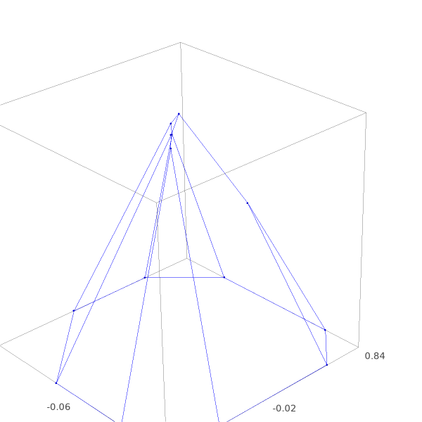
We can finally use this visualization tool to illustrate what happens with the perturbation strategy for handling linear dependency. We perturb vector $b$ by quite a lot for visualization purposes. In practise, one would work with much smaller perturbations

p = Polyhedron(ieqs = [[0,0,0,1],
                       [0.81,-1,0,-1],
                       [0.93,1,0,-1],
                       [0.84,0,-1,-1],
                       [0.87,0,1,-1],
                       [0.88,-s,s,-1],
                       [0.82,s,s,-1],
                       [0.96,s,-s,-1],
                       [0.95,-s,-s,-1]])

g = p.plot(fill=False)
g.save('tmp2.png', zoom=1.5, figsize=[6, 6])
Image(filename='tmp2.png')

The point of the pyramid has split into multiple vertices, each one being the intersection of 3 planes in stead of 8. Each one being non-degenerate.

Back to handling linearly dependent constraints

The discussion on handling linearly dependent constraints in an active set method, I’d like to finish with a shoutout to qpOASES. qpOASES is one of the best open source QP solvers out there. It is supported by the COIN-OR initiative, which is a testament to its quality. Moreover, it has its roots with one of my favorite professors when I studied in Leuven (prof. Moritz Diehl), so that does make me biased.

OASES stands for ‘Online Active Set Strategy’, which actually refers to its ability to do hotstarting on multiparametric quadratic programs with changing constraints (which makes hotstarting nontrivial). This is very suited for Model Predictive Control applications.

So qpOASES is a very cool and smart method, but when used as a basic QP solver, it behaves quite a lot like your typical active set method, albeit a very decent implementation. The qpOASES paper details out quite extensively how it deals with ‘ties’ and degeneracy. My experience with qpOASES on real QPs with linearly dependent constraints (e.g. the sampled polynomial constraint example) has been very positive: It manages to converge without cycling.

Interior point methods

Finally, we come perhaps to the real conclusion: as interior point methods don’t work with the concept of active/inactive constraints, and as intermediate iterates of interior point method never lie exactly on the feasible set boundary, interior point methods quite naturally don’t have any problem with linearly dependent constraints. Because of the not-so-rare occurence of these types of constraints, when implementing a constrained solver from scratch, interior point methods are much easier to get robust.

Related posts

• A much nicer constraint visualization tool

Want to leave a comment?

Very interested in your comments but still figuring out the most suited approach to this. For now, feel free to send me an email.